Sea Ice Sensitivity

Overview

This recipe and diagnostic calculates the rate of sea ice area loss per degree of warming, as in plot 1d of Notz et al. and figure 3e of Roach et al.. The figures used in the plots are output to csv files in the work directory.

Available recipe and diagnostic

Recipe is in recipes

• recipe_seaice_sensitivity.yml

Diagnostic is in diag_scripts/seaice/

• seaice_sensitivity.py (Plotting the sensitivity of sea ice to mean global temperature).

Recipe settings

Years to be evaluated are specified with the start_year and end_year keywords in the model dataset section, which are automatically duplicated into the observational datasets section.

model_defaults: &model_defaults { ..., start_year: &data_start 1979, end_year: &data_end 2014}

Pre-calculated values for the mean sensitivity of sea ice area to global warming (and an associated standard deviation and plausible range) can be entered be for both arctic and antarctic diagnostics (more details are given in the “References” section below).

diagnostics:
  arctic:
    scripts:
      sea_ice_sensitivity_script:
        observations:
          observation_period:
            start_year:
            end_year:
          sea_ice_sensitivity:
            mean:
            standard deviation:
            plausible range:

If the years to be evaluated differ from those specified for pre-calculated observational values for either hemisphere, then the “observational period” is assumed to be a subset of the dataset evaluation period and all statistics will be calculated for both periods, with these results shown as two halves of the sensitivity (one dimensional) plot. The two dimensional plot will only use values from the entire evaluation period.

Arctic sea ice is evaluated using data from September, and Antarctic sea ice is evaluated using annually meaned data. This can be amended by changing the preprocessor for each variable (shown below).

pp_arctic_sept_sea_ice:
  extract_month:
    month: 9
  extract_region:
    start_longitude: 0
    end_longitude: 360
    start_latitude: 0
    end_latitude: 90
  area_statistics:
    operator: sum
  convert_units:
    units: 1e6 km2

Datasets

The recipe tries to use as many datasets as possible from the list in Table S3 of https://agupubs.onlinelibrary.wiley.com/action/downloadSupplement?doi=10.1029%2F2019GL086749&file=grl60504-sup-0002-Table_SI-S01.pdf Only one ensemble member is used for each model.

All, some or no datasets may be labelled in the plots, using label_dataset: True in the recipe settings.

Note

The same time range must be used for all observational datasets specified.

This is because the linear regression of sea ice area against temperature is calculated directly for some values in the plots, and so both types of observation must have the same number of data points.

References

• SIMIP_2020: Scripts for the processing, analysis and plots of the SIMIP Community Paper (Notz et al. 2020), jakobdoerr/SIMIP_2020

Example plots

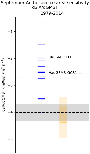
Fig. 396 Plot of sensitivity of northern hemisphere sea ice area loss (millions of square kilometres) in the month of September to the annual mean global temperature change (K). Models are shown on the left in blue, and the relationships between SIA-GMST pairs of observational datasets are shown on the right in orange. The shading around the position of each observational pair shows the standard error as computed by scipy.stats.linregress().

The dashed black line shows the observational mean, the shaded area denotes one one standard deviation of observational uncertainty, as calculated by Notz et al (2020). The dotted grey lines reflect Notz et al estimate of a plausible range incorporating both internal variability and observational uncertainty. These values are configurable in the recipe, with the default values taken from Notz et al (2020):

mean	-4.01 million km2 K-1
std_dev	0.32 million km2 K-1
plausible	1.28 million km2 K-1

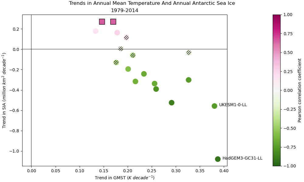
Fig. 397 Plot of the trend of annually averaged southern hemisphere sea ice area (millions of square kilometres) over time against the trend of annually and globally averaged air temperature near the surface (degrees Kelvin) over time. The values plotted are 10 times the annual trend, which was calculated using scipy.stats.linregress(), for consistency with the decadal values used in the published plot.

The colour of each point is determined by the Pearson correlation coefficient between the two variables, and the hatching indicates that the trend of sea ice area over time has a p_value greater than 0.05, both calculated using scipy.stats.linregress(). Models are shown as circles and observational datasets are shown as squares.